Meta-analysis

Scientific studies often disagree with each other - effects measuring the same thing may have different magnitudes or different directions altogether. Meta-analysis is a statistical tool that aims to resolve these discrepancies and, ideally, explain them.

Note

This section is a read-along, not a code-along - some code is hidden so you won’t be able to run it. The first “proper” tutorial starts in the next section.

How is meta-analysis like a linear model?

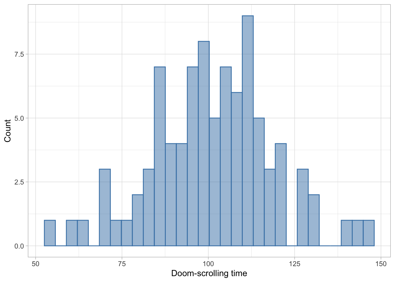
In its most basic form, a meta-analysis gives us “typical value” for an effect, much in the same way a linear model gives us a typical value on some variable measured in a sample. Imagine we collected a sample of participants and measured their doom-scrolling habits. We could end up a sample like this:

To find out how much a typical individual doom-scrolls, we could calculate the mean (or some robust alternative if we’re worried about outliers):

mean(doom, na.rm = TRUE)

[1] 101.1701

This is the same as fitting a linear with no predictors - a null model that predicts the outcome only from an intercept:

lm(doom ~ 1) |> 
  model_parameters() |> 
  display()

Parameter	Coefficient	SE	95% CI	t(89)	p
(Intercept)	101.17	1.87	(97.46, 104.88)	54.15	< .001

In a meta-analysis, our outcome is the effect size that represents a hypothesis. Say that we measured the doom-scrolling habbits of students and compared them to the doom-scrolling of lecturers. We could fit a linear model with the group as the predictor:

doom_lm <- lm(doom ~ group, data = doom_tib)

doom_lm |> 
  model_parameters() |> 
  display()

Parameter	Coefficient	SE	95% CI	t(98)	p
(Intercept)	122.35	2.55	(117.28, 127.41)	47.92	< .001
group (Student)	-21.34	3.61	(-28.50, -14.17)	-5.91	< .001

Which tells us that students doom-scrolling time was on average lower by -21.34 minutes, compared to the lecturers. This value is our effect size. We could convert it into a standardised effect like a standardised beta to make it comparable to other studies who may have used a different way of operationalising the doom-scrolling measure:

doom_lm |> 
  model_parameters(standardize = "refit") |> 
  display()

Parameter	Coefficient	SE	95% CI	t(98)	p
(Intercept)	0.51	0.12	(0.27, 0.75)	4.18	< .001
group (Student)	-1.02	0.17	(-1.36, -0.68)	-5.91	< .001

More often than not, you might see the effect size reported as “Cohen’s d” which is another way of expressing a standardised difference:

effectsize::cohens_d(doom ~ group, data = doom_tib)

Cohen's d |       95% CI
------------------------
1.18      | [0.75, 1.60]

- Estimated using pooled SD.

We could then try to find all the papers that have ever measured doom-scrolling and compared students and lecturers. Each would report a standardised effect size representing the difference (or we could calculate it based on what’s reported in the paper). When we collate these effect sizes, we could end up with something like this:

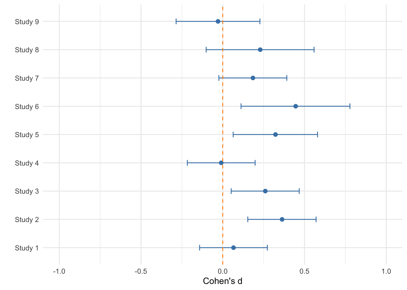
In the plot above, the dots represent the effect sizes from different studies and the error bars are their confidence intervals. We can see that the majority of the studies indicate a positive difference (lecturers doom-scroll more than students), but several of the confidence intervals include zero as well as negative values.

In a very crude fashion, we could calculate the average effect size:

cohen_lm <- lm(Cohens_d ~ 1, data = doom_d)

cohen_lm |> 
  model_parameters() |> 
  display()

Parameter	Coefficient	SE	95% CI	t(8)	p
(Intercept)	0.20	0.06	(0.08, 0.33)	3.67	0.006

Based on this, we could conclude that on average, lecturers scroll more than students, with an overall small effect size (Cohen’s d = 0.2).

Of course, there’s more to meta-analysis than that. For example, we need to account for the fact that:

Some studies only have a handful of participants others have loads
The intervals around some effect sizes are wider compared to other studies (i.e. there is more uncertainty associated with them)
If the effect sizes vary substantially, are there any predictors that can explain this?
Some studies may have operationalised outcome as a binary variable (“Doom-scrolls” vs “Doesn’t doom-scroll”), resulting in an odds ratio as an effect size - is there a way to include these studies in the same analysis, and does it make sense to do so?
Some studies reported means, standard deviations and sample sizes, allowing us to calculate Cohen’s d directly. Others only reported the t or the F statistics, or just the p-value - how can we calculate the effect size for them?
Some studies report multiple effect sizes - do we include them all, even though they are dependent?
What about studies that never made it to the publication stage? Could they change our conclusion if we were to include them?

A well-conducted meta-analysis can address these questions and we’re going to learn how in the weeks to come.

Reading list

The tutorials will focus on the practical aspect of data wrangling and fitting meta-analytic models, while the book chapter associated with this block explains the theoretical aspects of conducting a meta-analysis in more detail.

Essential reading

The book chapter will be linked to the weekly pages under Units on Canvas. You can therefore access it through:

Units > Week 4
Units > Week 5
Units > Week 6

This book chapter is essential reading . You should aim to finish reading the chapter by the session in Week 6, at which point we’ll start working on the Report together.

How is meta-analysis like a linear model?

Reading list

Essential reading

Further reading